Continuous distribution family

Yu Cheng Hsu, PhD

Intended learning outcomes

• Identify key properties of Normal and \(\chi^2\) distributions.
• Understand the application of conjugate priors in Bayesian estimation for Normal parameters.
• Apply Markov’s and Chebyshev’s inequalities to bound probabilities.
• Explain the Law of Large Numbers (LLN) and Central Limit Theorem (CLT) and their implications for statistical inference.

Normal distribution

If a random variable follows a normal distribution: \(X \sim N(\mu,\sigma^2)\)

Properties

• Support \(x \in \mathbb{R}\)
• Parameter \(\mu, \sigma\)
• pdf

\[ f_X\left( x \right) = \frac{1}{\sqrt{2\pi\sigma^2}}e^{-\frac{(x-\mu)^2}{2\sigma^2}} \]

The Binomial distribution approximates the normal distribution when \(np\) and \(n(1-p)\) are large enough (usually \(\ge 10\)).

Since the Poisson distribution can approximate the Binomial, it can also approximate the Normal distribution under large \(\lambda\).

\(\chi^2\) distribution

Let \(Z_1, \dots, Z_k\) be independent standard Normal variables. Let \(V=\sum_{i=1}^k Z_i^2\). Then \(V\) follows a \(\chi^2\) distribution with \(k\) degrees of freedom: \(V \sim \chi^2(k)\).

Properties

• Support \(x \in [0;+\infty)\)
• Parameter \(k\)
• pdf \[ f_X\left( x \right) = \frac{1}{2^{\frac{k}{2}}\Gamma(\frac{k}{2})}x^{\frac{k}{2}-1}e^{-\frac{x}{2}} \]

• \(\chi^2\) distribution is a special case of Gamma distribution where \(\lambda = \frac{1}{2}\) and \(\alpha=\frac{k}{2}\)

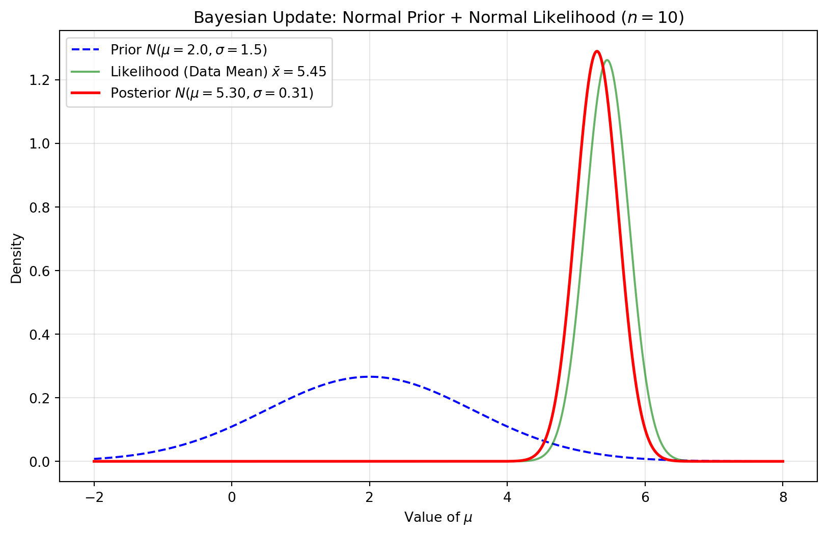
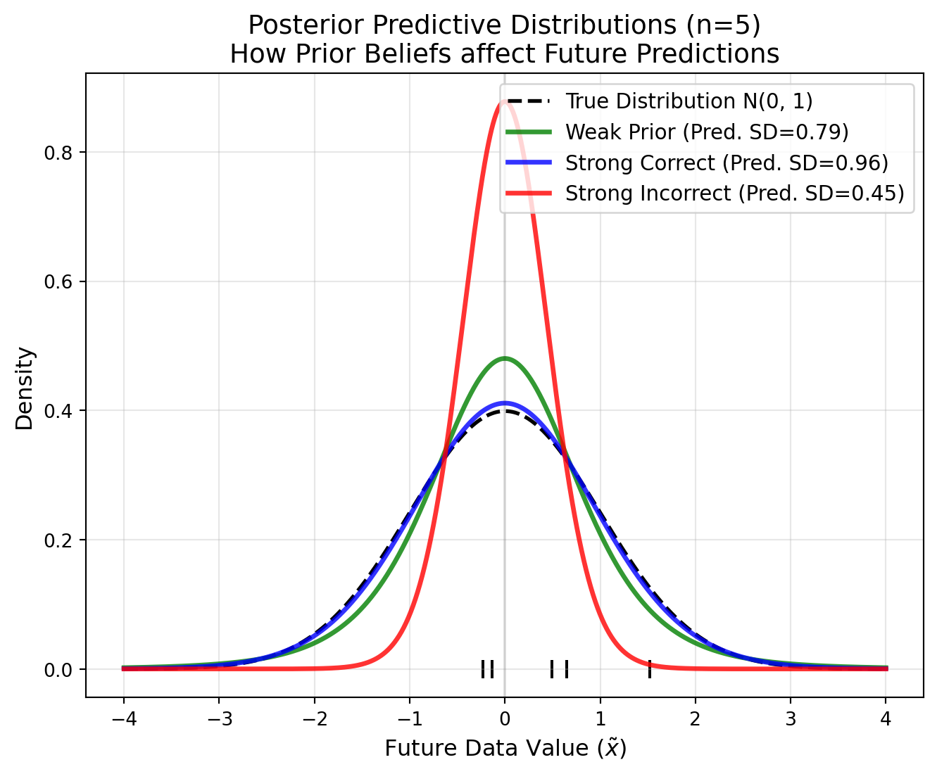
Prior on mean

• The Normal distribution is the conjugate prior for the mean \(\mu\) (given known \(\sigma^2\)). Consider IID observations \(x_i \sim N(\mu, \sigma^2)\) where \(\sigma^2\) is known. If the prior is \(\mu \sim N(\mu_0,\sigma^2_0)\):

• Posterior: \(\mu' \sim N\left(\frac{\frac{n\bar{x}}{\sigma^2}+\frac{\mu_0}{\sigma^2_0}}{\frac{n}{\sigma^2}+\frac{1}{\sigma^2_0}}, \left(\frac{n}{\sigma^2}+\frac{1}{\sigma^2_0}\right)^{-1}\right)\)

• The posterior predictive distribution follows \(p(\tilde{x}|X)\sim N(\mu', \sigma^{2'} + \sigma^2)\)

• Interpretation: The posterior mean is a weighted average of the prior mean and the sample mean, weighted by their respective precisions.

Prior on variance

• The Gamma distribution is the conjugate prior for the precision \(\lambda = \frac{1}{\sigma^2}\). Consider IID observations \(x_i \sim N(\mu, \sigma^2)\) where \(\mu\) is known. Let the prior be \(\lambda \sim \text{Gamma}(\alpha, \beta)\).

• Posterior: \(\lambda \sim \text{Gamma}\left(\alpha + \frac{n}{2}, \beta + \frac{\sum_{i=1}^n (x_i - \mu)^2}{2}\right)\)

• Interpretation: The prior acts as if we had \(2\alpha\) prior observations with a sum of squared deviations equal to \(2\beta\).

• The posterior predictive distribution follows a non-standardized Student’s t-distribution.

Inequalities, convergence, and law of large number

Preface

This section covers properties of probability bounds and convergence. These are helpful for:

• Knowing the estimation boundary
• Understanding how estimators behave as sample size increases.

On the other hand, the mathematical proof for this part is relatively simple (and brings little insight to our practice) So we will only cover the intuition and implication of these properties, and leave the mathematical proof to the tutorial questions.

Markov’s inequality

• Let \(X\) be a non-negative r.v. and suppose \(\mathbb{E}(X)\) exists. For any \(t>0\)

\[ P(X>t)\leq\frac{\mathbb{E}(X)}{t} \]

Implication

• Extreme events are:
  • Rare
  • Bounded by the mean
    
  • The probability of an event decays at least inversely proportional to its magnitude.

Example question If the average survival time for a specific cancer is 5 years, what is the upper bound of the probability of a patient surviving more than 20 years?

0.25 = 5/20

Chebyshev’s inequality

• Let \(\mu=\mathbb{E}(X)\) and \(\sigma^2=\mathbb{V}(X)\), then:

\[ P(|X-\mu|\geq t)\leq\frac{\sigma^2}{t^2} \]

or in the other words

\[ \small P(|Z|\geq k)\leq\frac{1}{k^2}, \text{ where } Z=(X-\mu)/\sigma \]

A clear bound for outliers:

Deviations (k)	Chebyshev Guarantee (Minimum)	Normal Distribution (Actual)
2 σ	At least 75% inside	95.4% inside
3 σ	At least 89% inside	99.7% inside
5 σ	At least 96% inside	99.9999% inside

• These inequalities allow for quick sanity checks on statistical claims without assuming a specific distribution.

Convergence

Convergence studies the behavior for a series of IID random variables \(X_1, X_2, \dots, X_n\) with CDF \(F_n\), while Let \(X\) be another r.v.s, with CDF \(F\). There are three types of convergence

1. \(X_n\) converges to \(X\) in qudratic mean \(X_n \xrightarrow{qm} X\) if \[ \mathbb{E}(X_n-X)^2\rightarrow 0 \]
2. \(X_n\) converges to \(X\) in probabiliity \(X_n \xrightarrow{P} X\) if, for every \(\epsilon>0\) \[ \mathbb{P}(|X_n-X|>\epsilon)\rightarrow 0 \]
3. \(X_n\) converges to \(X\) in distribution \(X_n \leadsto X\) if \[ \lim_{n\rightarrow\infty}F_n(t)=F(t) \]

Weak Law of large numbers (WLLN)

Let \(X_1, \dots, X_n\) be IID with \(\mathbb{E}(X_i) = \mu\) and \(\mathbb{V}(X_i) = \sigma^2\). The sample mean is \(\bar{X}_n = \frac{1}{n}\sum X_i\).

WLLN states

\(\bar{X}_n \xrightarrow{P} \mu\) as \(n \to \infty\).

• Implications
  • Probability as long-run frequency: The core of the Frequentist perspective.
  • The variance of the sample mean, \(\frac{\sigma^2}{n}\), shrinks as \(n\) increases.
  • Larger datasets provide more accurate parameter estimates.

Bayesian perspective of probability

• Probability is a degree of belief, which can be updated by new evidence.
• Parameters themselves are random variables, estimated using data and prior beliefs.

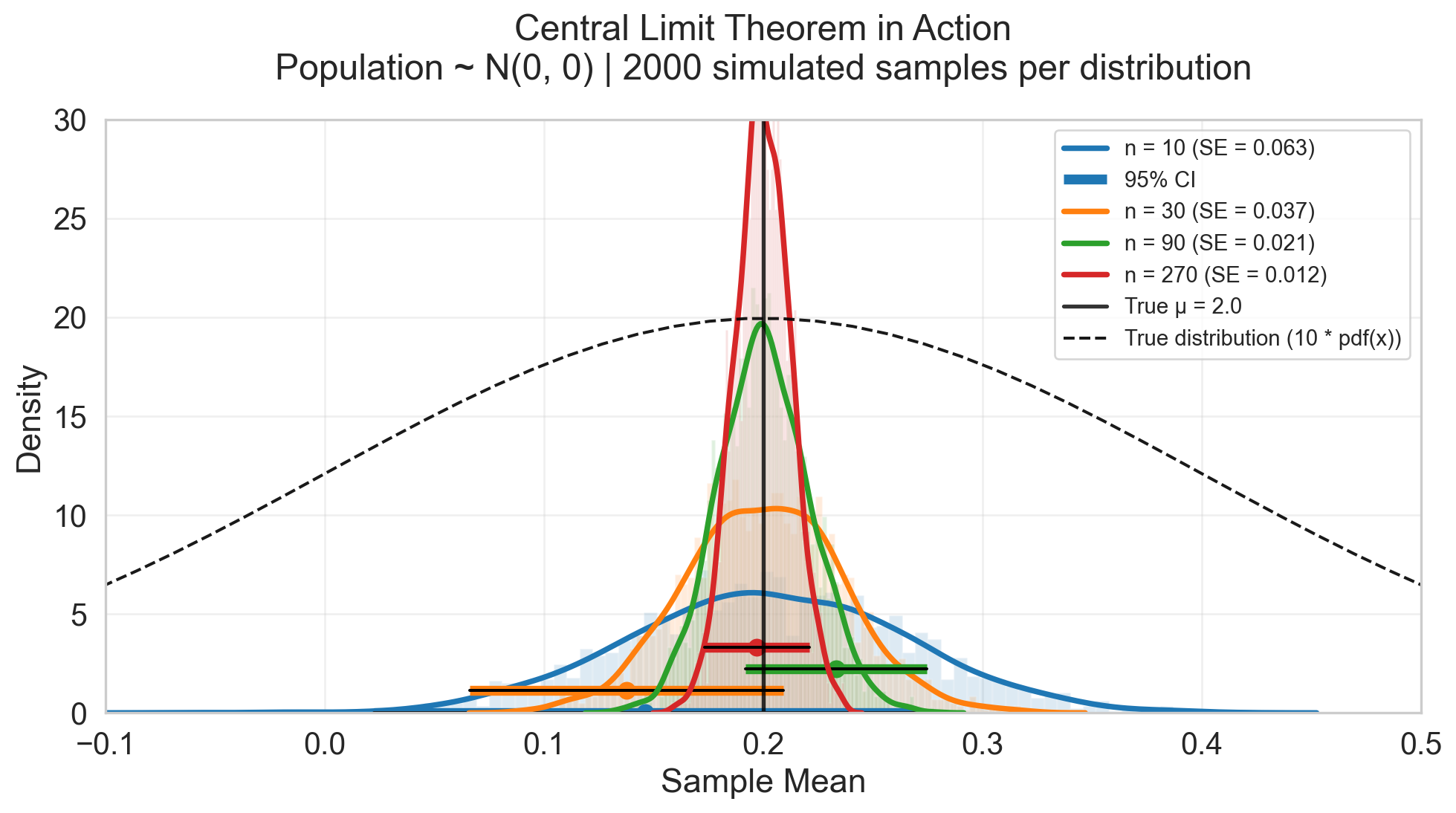
Central limit theorem (CLT)

Theorm

Let \(X_1, X_2, \dots, X_i\) be a sequence of iid random variables with mean \(\mu\) and variance \(\sigma^2\). The sample mean of the observarion \(\bar{X}_n=\frac{\sum_i^n X_i}{n}\), then

\[ \small \bar{X}_n \leadsto \text{Normal}(\mu, \frac{\sigma^2}{n}) \]

Implication

• Great sample size provide accurate estimation to “population mean”
• The marginal benefit of increasing sample size decreases (due to the \(\sqrt{n}\) term).
• Distribution-free: The sample mean becomes normal regardless of the underlying distribution (given finite variance).
• Foundation for hypothesis testing and confidence intervals.

Equivalent Statements

Define \[ \small Z = \frac{(\bar{X}_n - \mu)}{\sigma / \sqrt{n}} . \]

then the following statements are equivalent to CLT \[\begin{aligned} \small Z \leadsto N(0,1) \\ \bar{X}_n -\mu \leadsto N(0, \frac{\sigma^2}{n})\\ \sqrt{n}(\bar{X}_n -\mu) \leadsto N(0, \sigma^2)\\ \end{aligned} \]

Tip: Any proper algebraic transformation applied to both sides results in a valid equivalent statement.

Curse of big data

When the sample size is extremely large, almost any tiny difference becomes “statistically significant” (\(p < 0.05\)).

Reason

• The Standard Error (\(\sigma/\sqrt{n}\)) becomes so small that the confidence interval is incredibly narrow.
• Even biologically irrelevant differences can reject the null hypothesis.

Implication

• Distinguish between statistical significance and clinical/scientific significance.
• Effect size becomes more important than p-values in large datasets.

Curse of big data

We try to estimate the true \(\mu\) from a population \(N(0.2, 0.2^2)\).

• As \(n\) goes greater, we can estiamte the mean more accurately
• \(P(x\leq 0) = 0.15\) You might observe observations less or equal to 0
• You can still have an accurate estimation of truen men 0.2, which different from zero
• Does this 0.2 difference from 0 so important?